Autodiff performance and validation

Requires the jax extra: pip install 'clerq[jax]'. See AutodiffPropagation for the API.

This page records measurements of the released clerq.autodiff (0.14.0): what a gradient costs, how much memory it needs, how accurate it is, and what it buys on a design problem. The harness that produced every number is in benchmarks/autodiff/ (with the raw results in benchmarks/autodiff/results/), so they can be reproduced and rerun on other hardware.

One machine, CPU only

All timings are on one Apple M1 Max (10 cores, 64 GB, macOS 26.6.2) on AC power, CPU only, Python 3.14.4, JAX 0.11.2, diffrax 0.7.2. Other applications were running, so the one-minute load average was 2 to 8 (median 3 to 5) during the runs; the runs of different methods are interleaved so that drift affects them alike. The cost cells are the median of 7 repeats after warm-up (5 in the before-and-after comparison, 3 for the slowest), with a bootstrap 95% interval of the median in the harness output; the memory and compile-time cells are the best of two or three calls in a fresh process. No GPU was used, and the ratios (gradient cost over forward cost, autodiff over finite differences) are the portable part; absolute seconds are not.

The cost of a gradient

A reverse-mode gradient costs about six forward propagations, whatever the number of parameters. The parameters here are the coefficients of a free-form probe control (a Gaussian basis, see clerq.autodiff.controls), so N can be varied freely.

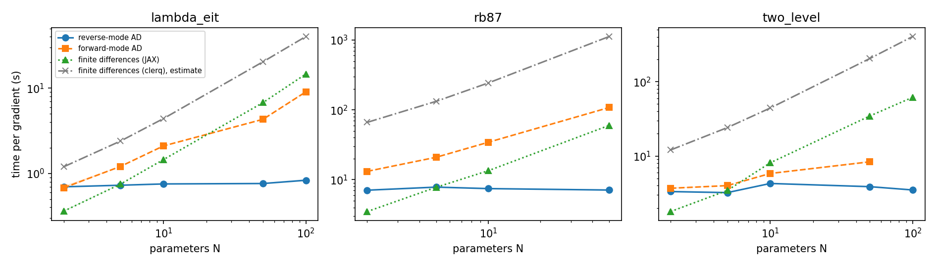
Time of one gradient against the number of parameters

system	forward (s)	reverse (s)	reverse / forward	at N = 50: forward-mode (s)	finite differences, JAX (s)	finite differences, clerq (s, estimated)	reverse speed-up over JAX / clerq
two-level, 1001 × 200	0.68	3.9	5.7	8.4	34.6	205	8.9x / 53x
lambda, 3 levels, 201 × 60	0.13	0.76	5.8	4.3	6.8	20.4	8.9x / 27x
Rb87, 11 levels, 11 classes, 201 × 50	1.18	7.1	6.0	108	60	1130	8.4x / 158x

At N = 100 (two-level and lambda) the speed-up over finite differences through JAX is 17.7x and 17.6x, and over clerq 116x and 48x.

What the finite differences are. Forward differences, N + 1 evaluations, through the compiled propagation. Central differences cost twice as much, which doubles every speed-up here. The finite differences through clerq are an estimate: N + 1 times the measured time of one PropagationSolver.solve() (4.0 s, 0.40 s and 22 s for the three systems), not a measurement of that many solves.
When reverse mode wins. It costs the same as finite differences through JAX at about N = 5, and is faster from N = 10 (1.8x to 1.9x on all three systems).
Forward mode (mode="forward") was never faster than reverse mode: equal at N = 2 on the lambda system and slower elsewhere (for example 13 s against 7 s for Rb87 at N = 2), and its cost grows with N. It was skipped for the two-level system at N = 100, where it would have taken over two minutes.
First call. The first call includes compilation: a forward propagation takes 1.4 to 2.4 s the first time and the reverse-mode gradient 5.5 to 12 s, against steady-state times of 0.13 to 1.2 s and 0.74 to 7.5 s. A new array shape or loss function recompiles, so pass the same loss object between calls.

Memory

Plain reverse mode through the z scan (strategy s2) stores every slice, so its memory grows with the number of z steps and of velocity classes. The default (s3) recomputes a slice on the backward pass and s4 also limits the solver’s inner checkpoints (here to 32). The figure shows the temporary memory XLA reports for one compiled gradient.

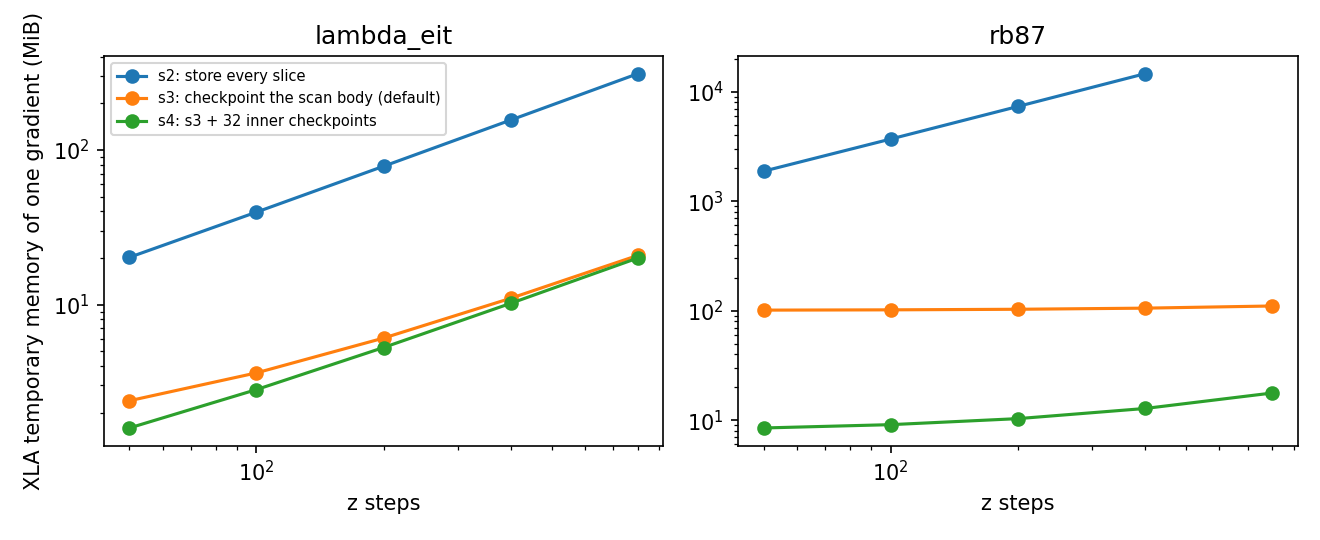
For Rb87 with 11 classes and 400 z steps, s2 needs 14.3 GiB, s3 105 MiB and s4 13 MiB; at 800 z steps s3 needs 110 MiB and s4 18 MiB (s2 was not run). For lambda at 800 steps it is 312 MiB, 21 MiB and 20 MiB. Against the number of classes (Rb87, 100 z steps, 1, 11 and 25 classes): s2 347, 3698 and 8391 MiB; s3 11, 102 and 229 MiB; s4 2, 9 and 19 MiB. Checkpointing costs time: the steady-state gradient is about 20% slower with s3 than with s2 and 26% to 39% slower with s4 (Rb87, 100 z steps, 11 classes: 15.0 and 15.8 s against 12.5 s; lambda at 100 z steps: 1.28 and 1.46 s against 1.05 s).

The peak resident set of the process also includes JAX and compilation, about 380 to 600 MiB above the baseline for s3 and s4 whatever the problem, so the XLA figures are the ones that separate the strategies.

Accuracy

system	N	fixed steps	field error against `solve()`	AD against finite differences	forward against reverse	adaptive against fixed-step AD
two-level	10	2003	2.5e-4	8.0e-9	8.5e-14	2.5e-5
lambda	10	2003	8.9e-8	2.3e-12	1.1e-16	1.9e-7
Rb87, 11 classes	6	1009	3.6e-4	5.4e-13	6.5e-16	4.8e-8

(The Rb87 case is smaller than the others because a fixed-step reference with 11 classes is slow.)

The gradient is the exact gradient of the discretised problem: it agrees with central finite differences on a fixed-step solve to 8e-9 or better (best of four step sizes: the two-level problem needs steps of 1e-7 or smaller because its loss is very nonlinear), and forward and reverse mode agree to 1e-13 or better.
The propagated field agrees with solve() to 2.5e-4 of the peak for the two-level problem and 3.6e-4 for Rb87 at the grids used here, and to 9e-8 for the lambda problem. We did not isolate the cause of the two larger differences, and the error did not fall steadily when the time grid was refined for the two-level problem.

Precision

clerq.autodiff computes in whatever precision JAX is set to: float32 by default, float64 with jax.config.update("jax_enable_x64", True). Float64 is the reference. The default solver tolerances follow the precision (rtol, atol of 1e-8 and 1e-10 in float64, 1e-6 and 1e-9 in float32, whose machine epsilon is 1.2e-7). Each problem was run in a fresh process in each precision at its default tolerances (benchmarks/autodiff/e8_precision.py, 10 control coefficients); the errors are of the float32 result against the float64 one.

problem	field error	loss error	gradient error	forward: float64 / float32 (s)	gradient: float64 / float32 (s)
two-level	1.4e-5	5.4e-8	4.8e-5	0.76 / 0.35 (2.1x)	4.36 / 2.35 (1.9x)
lambda	1.3e-6	4.0e-7	1.2e-6	0.14 / 0.09 (1.6x)	0.81 / 0.49 (1.7x)
Rb87, 11 levels, 11 classes	2.1e-5	6.7e-7	6.4e-7	1.27 / 0.91 (1.4x)	7.64 / 5.48 (1.4x)
lambda, 400 z steps	8.4e-6	1.6e-6	3.2e-6	1.21 / 0.92 (1.3x)	6.88 / 4.60 (1.5x)
lambda, 4000 time points	2.7e-6	9.5e-7	2.9e-6	0.55 / 0.52 (1.1x)	3.08 / 2.38 (1.3x)

The field error is the largest difference over all fields, z slices and times, relative to the peak. The errors do not grow along a long z march or a fine time grid.
Most of the difference is the solver tolerance, not the precision: in float64 with the float32 tolerances (1e-5, 1e-7) Rb87 shows the same 2.1e-3 field error. Float32 with the float64 tolerances (1e-8, 1e-10) still agrees to about 1e-6, but gains little or no speed, and the two-level pulse took twice as long because the step controller cannot meet a tolerance below the precision.
Where the loss is close to zero float32 gradients are noisier: at a random start of the memory design problem, where only 4e-8 of the pulse is retrieved, the 44-parameter gradient differed by 6e-3. Thirty Adam steps from there followed the float64 trajectory to 1e-3 (final 0.4296 against 0.4298).
Use float64 for finite-difference checks (which need it), for tolerances tighter than about 1e-6, and for results quoted as reference values.
Not tested: optical depths well above 25, stiff systems, and a CUDA GPU. On a consumer GPU float32 is the precision that runs at full speed.

The Apple GPU

With float32 the Apple GPU can run the backend, with a plugin that tracks JAX 0.11 (jax-mps, on MLX; one run on an M1 Max with jax-mps 0.11.1 and diffrax 0.7.2, not part of the harness). Complex64, scans, gradients through a checkpointed scan and diffrax solves, including their reverse and forward-mode gradients, all worked once EQX_ON_ERROR=nan was set (without it diffrax’s error check needs a host callback that the plugin does not provide). Fields agreed with the CPU in float32 to 1e-6 and gradients to 6e-5. It was far slower, though: a 40-point, 4-slice lambda forward took 10 to 12 s against under 5 ms on the CPU, and the first gradient of a 60 by 6 problem 140 s against 5 s. Each operation inside a loop costs 4 to 9 microseconds there against 0.02 on the CPU (no fusion), so the time scales with the number of operations the solver executes. It stayed nearly flat as the number of velocity classes grew (9.6 s at 11 classes, 11.3 s at 401), so by extrapolating the CPU’s linear growth it would overtake the CPU only at a few thousand classes. It is useful as a correctness check on a second backend, not as a speed-up.

A design problem

The memory problem in the research notes: store a probe pulse in a Doppler-broadened lambda medium (11 classes, effective optical depth about 25) with the coupling field off, and maximise the energy retrieved afterwards. A 5-parameter baseline (a super-Gaussian probe and two coupling amplitudes) searched with Nelder-Mead is compared with a free-form design of 44 coefficients by gradient descent (Adam).

A 44-parameter gradient took 36 s with reverse mode against 279 s with forward differences (one forward evaluation takes 6.2 s).
The baseline reached 0.068 retrieved after 296 evaluations and 2261 s.
The free-form design passed that value at step 23, after 1037 s, and reached 0.106 after 40 steps (1809 s). With finite-difference gradients the same 23 steps would take about 6400 s (an estimate from the measured gradient time).

This run was slower than earlier runs of the same problem on the same machine (a forward evaluation took 3.2 s in earlier runs); we did not identify why. The ratios are within a run. It is one problem, one optical depth and one Doppler width. Without Doppler broadening a tuned three-parameter baseline matched the free-form result in the research notes (0.469 against 0.460), so this advantage should not be assumed for other problems.

Against gradient-free search at equal cost

A gradient is expensive to compute (about six forward evaluations), so the fair question is whether a search that uses it beats a gradient-free one given the same total cost. The same design problem without Doppler classes (optical depth 25, 44 parameters, benchmarks/autodiff/e7_equal_cost.py) was given a budget of 550 objective evaluations, 12.5 per parameter, with a gradient call charged at the measured 6.5 evaluations. Three random starts each; the retrieved fraction at the end of the budget:

optimiser	per seed	median
Adam, exact gradients	0.459, 0.439, 0.447	0.447
L-BFGS-B, exact gradients	0.000, 0.462, 0.000	0.000
CMA-ES	0.399, 0.385, 0.404	0.399
differential evolution	0.315, 0.336, 0.299	0.315
Latin hypercube	0.250, 0.259, 0.232	0.250

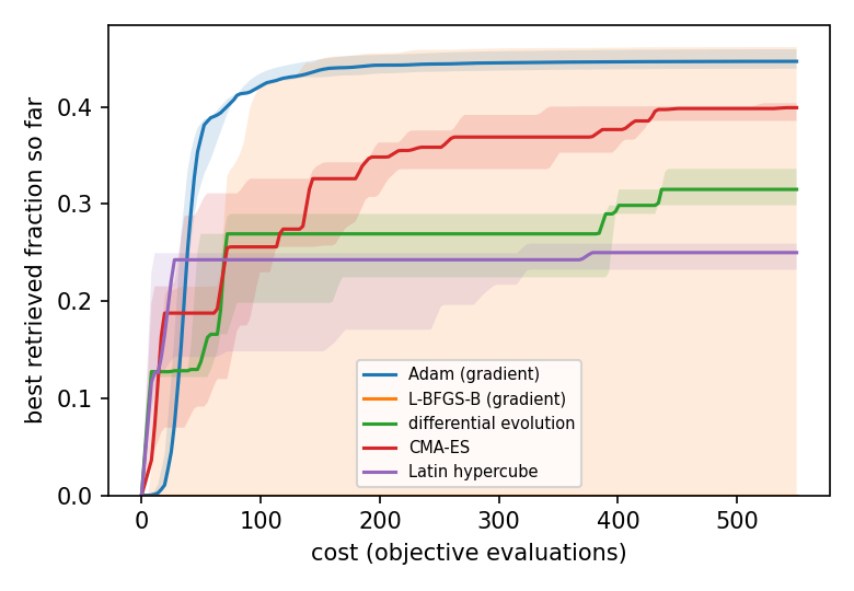
At equal cost the gradient search with Adam finished 12% above CMA-ES, the best gradient-free search, and 42% above differential evolution, on all three seeds. The margin over CMA-ES is modest. On the first seed Adam had reached 99.5% of its final value by half the budget, while CMA-ES and differential evolution had flattened by 80% of it.
L-BFGS-B found the best single control (0.462), but stopped after the first gradient call on two of the three seeds: the random starts retrieve only 3e-9 to 4e-8, and on those two the largest gradient component (5e-6 and 4e-6) is below L-BFGS-B’s default stopping threshold of 1e-5. Gradient methods need a start that retrieves something, or a method that does not stop on a tiny gradient (Adam does not).
This is one problem, 3 seeds and one budget (12.5 per parameter); neither CMA-ES nor differential evolution was tuned, so a tuned gradient-free search or a much larger budget might narrow the gap. A comparison by Lee (Zenodo 10.5281/zenodo.23407812, appendix) on a different memory problem found gradient search with L-BFGS-B below differential evolution at 16 and 32 control knots at a similar budget, with runs stopping at local optima, so the gradient’s advantage should not be assumed to carry over.
Wall times of these runs are not reported: other jobs shared the machine.

Cost of the decay-rate parameters

Adding decay_rates (pull request 361) changed how the decays enter the solver. Running the same cost tests on the commit before it and the commit after it, back to back: reverse mode took 1.00 to 1.01 times as long, a forward propagation 1.00 to 1.02 times, and forward mode 1.00 to 1.08 times (the largest at the two-level and lambda systems with N = 10). The two runs were sequential, so slow drift cannot be excluded.

Practical notes

Validate against fixed-step finite differences. Finite differences through an adaptive solver are noise-limited (error floors near rtol / h), so a gradient check against them can disagree by orders of magnitude when the gradient is right. Use n_steps= with a step count that does not divide the output grid, and compare at several step sizes.
Avoid commensurate fixed steps. With diffrax 0.7, fixed steps that land exactly on output times can give wrong reverse-mode gradients. clerq raises an error for this case.
Resolve the z march. An insufficiently fine z_steps_inner at high optical depth makes the march unstable and the energies meaningless; this is a property of the propagation scheme, not of autodiff.
Free-form controls need a smooth parametrisation. One free value per time sample lets an optimiser exploit the time grid (see clerq.autodiff.controls).

Not yet established

GPU performance; counter-propagating fields; dense (non-single-element) dissipators at scale; stiff regimes; systems of more than 11 levels; the largest cells (nine levels with 50 velocity classes, and s2 at 800 z steps for Rb87), which were not run; and any finite-difference timing through clerq beyond the one-solve estimate.